

Introduction
The demands on optical bandwidth are greater than ever; however, the need to process ever larger amounts of data at high speeds sets challenging targets for current and next generation fiber-optic networks. Photonic integrated circuits (PICs) promise to revolutionize the optical network industry by enhancing the transmission capacity of optical fiber communications at reasonable cost. To achieve this goal, PICs are rapidly becoming more complex, involving an exponentially increasing number of components. In the past, a similar increase in complexity in electronic chip design drove the need for automation that encompasses and supports all levels of abstraction present in the design and verification of integrated electronic design [1]. Today, the increasing complexity of PICs is driving a similar need fully automated design systems [2-3].
Optical circuit verification is one of the key steps of the PIC design flow, and includes the simulation and analysis of optical circuits and components. Circuit simulation requires nonlinear transient analysis and scattering data analysis to capture the optical and electrical signal waveforms in the time domain and the frequency domain, respectively.
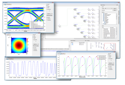
Figure 1: INTERCONNECT includes time and frequency domain simulation and analysis. Eye diagrams, time domain waveforms, transverse mode profiles and complex transmission spectra allow key parameters of the quality of the circuit to be determined.
Although photonic integration has much in common with electronic integration, a major difference is the variety of components and technologies in photonics. Lasers, modulators, couplers, filters and detectors are just a few of the different components present in a PIC. Furthermore, each one of these components has different operation principles and materials. Circuit simulations rely on proper compact models that accurately represent the optical and electrical responses of these components in time and frequency domain. Additionally, the optical simulation and analysis of PICs is particularly challenging because it also involves bidirectional, multichannel and even multimode propagation of light [4].
Software tools that can address these simulation challenges are a fundamental part of any PIC design flow. Lumerical’s INTERCONNECT [5] spans the entire PIC design flow, from system level to circuit level design and verification, including schematic capture, time and frequency domain simulations and analysis, and a comprehensive set of complex measurements on signal waveforms and transmission spectra. This white paper presents the different simulation approaches available in INTERCONNECT, and describes how the software models bidirectional, multichannel and multimode PICs.
Elements
INTERCONNECT photonic integrated circuits are composed of individual elements such as optical waveguides, phase modulators and photodetectors, linked by connections that transmit electrical and optical signals. Elements are the fundamental blocks of the circuit and they are represented by parameters and compact models. A ring resonator element, for example, can be modeled using an analytical equation or a scattering matrix. In both cases the compact model defines the relationship between the element’s input and output ports.
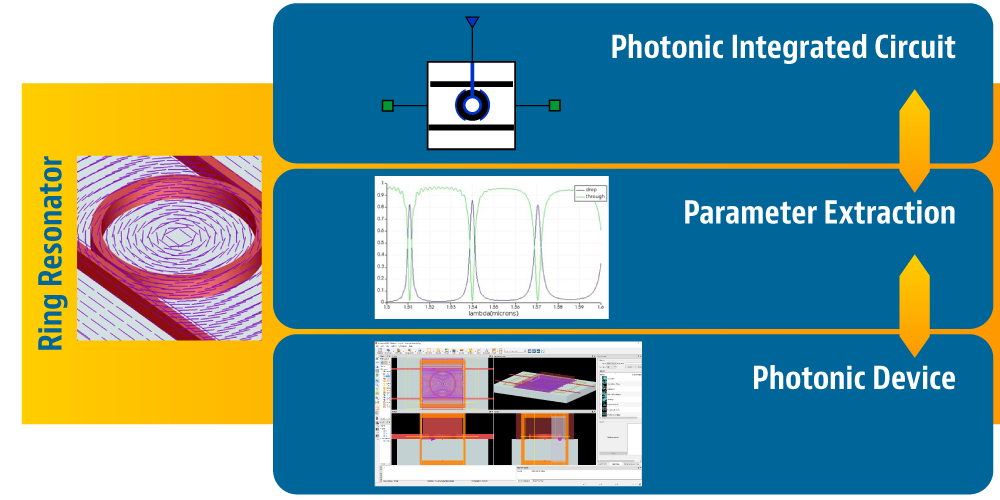
Figure 2: The FDTD method allows for solving Maxwell’s equations on finite difference mesh and extracting parameters such as the scattering matrix of a ring resonator. The extracted parameters can be fitted to an analytical model or used directly at the circuit level simulation.
The accuracy of the simulation is also defined by the quality of the compact model and its parameters. Parameter extraction is then a key process in this methodology. Using an eigenmode solver [6], waveguide propagation properties such as mode profiles, effective index, dispersion and loss can be extracted and then exported to a compact model of a waveguide element in the circuit. Similarly, the FDTD method [7] solves Maxwell’s equations on finite difference mesh: by analyzing the resulting fields, the scattering matrix of a component, e.g. a ring resonator, can be extracted. The parameter extraction itself can be potentially more complex in the optical domain than in the electrical domain. The potential multimode nature of optical waveguides implies that a scattering data approach is also more complicated than in the electrical domain.
Frequency Domain Analysis
INTERCONNECT frequency domain analysis is modeled on the same type of scattering analysis used in the high-frequency electrical domain for solving microwave circuits, enabling bidirectional signals to be accurately simulated [8]. However, it has been extended to allow for an arbitrary number of modes supported in the waveguide elements with possible coupling between those modes that can occur in any element. Consequently, the scattering matrix of a given element describes both the relationship between its input and output ports and the relationship between its input and output modes.
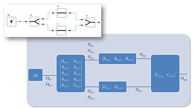
Figure 3: Block diagram of an INTERCONNECT circuit. Each element (A, B, C and D) is represented by a scattering matrix that defines the relationship between an arbitrary number of input and output ports and modes (y). IA is the circuit source and its output contains two modes.
Scattering analysis requires that the scattering matrix of each element in the circuit elements be known. This is not the case for circuits that contain opto-electronic devices, such as ring modulators, where the scattering matrix of the ring depends on its driving voltage. INTERCONNECT performs a preliminary simulation during which the circuit elements calculate their own scattering matrices. For example, the ring modulator can calculate its scattering matrix depending on the steady-state electrical signal input, enabling simulations of PICs containing both passive optical components and active opto-electronic elements. The preliminary calculation can also determine the coupling coefficients between two waveguides by performing overlap integration between waveguide modes before starting the scattering analysis, allowing the scattering matrix of a waveguide to combine its propagation properties and coupling losses into a single scattering matrix.
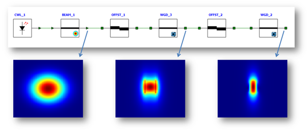
Figure 4: INTERCONNECT scattering data analysis includes the effects of coupling between different waveguides by taking into account each element’s transverse mode profiles.
INTERCONNECT frequency domain analysis of a circuit under test is performed by the Optical Network Analyze element (ONA), enabling the simultaneous analysis of multiple circuits in the same schematic. After the ONA runs the scattering data analysis of the circuit, a comprehensive set of measurements on the complex transmission spectra are calculated; typical results include gain, phase, dispersion and group velocity. Spectral peak analysis is also performed, which automatically calculates free spectral range (FSR), bandwidth, Q-factor, and other key parameters.
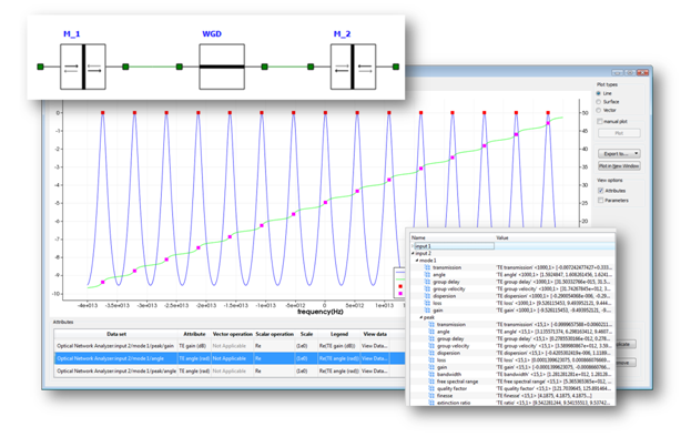
Figure 5: INTERCONNECT visualizer shows results of spectral and peak analysis on a Fabry-Perot resonator. Automatic peak detection and measurements provides comprehensive analysis of a device’s behavior.
The ONA can also perform parameter extraction by calculating and exporting the overall scattering matrix of a circuit under test. This total scattering matrix describes the complex transmission of the circuit under test. Once established, the circuit can be replaced by its equivalent scattering matrix element, improving simulation speed.
Time Domain Analysis
INTERCONNECT time domain analysis is performed using a dynamic data flow simulator. When a simulation runs, data flows from the output port of one element to one or more input ports of one or more connected elements. When an element receives data, its compact model applies its behavior to the data and generates the appropriate output. In the time domain simulation, data is represented as a stream of samples. Each sample represents the value of the signal at a specific point in time. S In addition to optical signals, INTERCONNECT supports digital and electrical signal types. This flexibility to represent different types of element behavior and signal types enables the development of compact models that can comprehensively address the variety of nonlinear opto-electronic devices present in photonic integrated circuits.
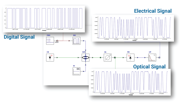
Figure 6: INTERCONNECT time domain simulation supports mixed-signal representation: digital, electrical and optical signals offers flexibility in handling the simulation at different levels of the integrated circuit.
Similar to the frequency domain simulations, the multimode nature of optical components is also included in the time domain simulation, and is not limited to two orthogonal modes or polarizations. INTERCONNECT optical signal support an arbitrary number of modes and base bands, giving designers the capability to simulate bidirectional, multimode and multichannel optical circuits.
INTERCONNECT relies upon Infinite Impulse Response (IIR) and Finite Impulse Response (FIR) digital filters to implement frequency dependent behavior in time domain simulations. For each signal mode and signal band, a corresponding digital filter is created, addressing complex single or multimode wavelength division multiplexing (WDM) devices. By supporting multiple baseband signals for coarse WDM circuits, one for each channel, different digital filters can be applied to different bands, reducing the limitations and trade-offs as to how well these digital filters can apply a desired frequency response to a time domain signal. Typical limitations are the ripple introduced by FIR filters due to the finite length of the impulse response. For instance, each scattering matrix in INTERCONNECT defines the relationship between an input and output signal mode, and each scatter parameter is defined by a vector of digital filters, where each filter is centered at the center frequency of the corresponding signal baseband.
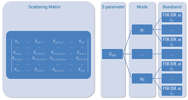
Figure 7: INTERCONNECT scattering matrix is a container of multiple modes and digital filters centered at each signal baseband.
INTERCONNECT time domain signal integrity analysis of a circuit under test is performed by analyzers connected to port monitors. Monitors are used to store the different signal types, and they can be placed at any output or bidirectional port of an element. As the simulation runs, analyzers can be added to the circuit and connected to the monitors allowing for real time analysis of simulation results. For instance, the eye diagram analyzer can perform a comprehensive set of measurements on the time domain waveform, including bit error rate (BER), optimum threshold and decision instant, and extinction ratio.
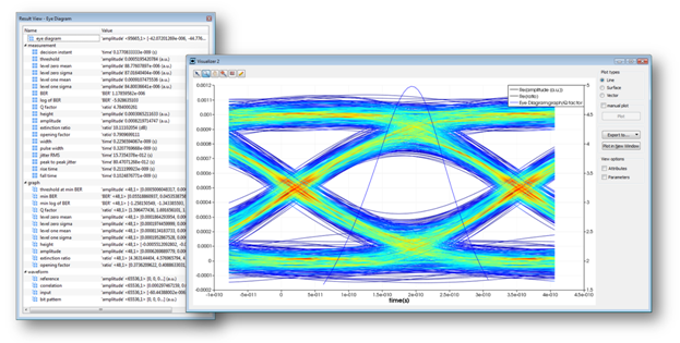
Figure 8: INTERCONNECT visualizer shows results of time domain analysis on an optical transceiver. The eye diagram analyzer offers insight into the nature of the circuit imperfections.
Example application: ring modulators
The ring modulator is a cavity working on the principle of the constructive interference of light inside a resonator, resulting in a tunable Lorentzian transfer function [9]. Frequency and time domain simulations are required to determine the optimum operation point of the device, and its influence on the overall circuit performance.
For the maximum modulation efficiency, the modulator is typically biased at the largest slope of the transfer curve. Frequency domain simulation, driven by the INTERCONNECT optical network analyzer, determines the operation frequency and bias of the modulator that maximizes efficiency. For a given bias voltage, the steady-state frequency response of the device can be determined and key metrics such as free spectral range, Q-factor and extinction ratio can then be calculated.
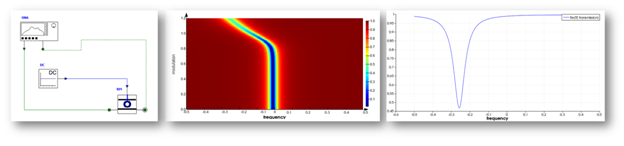
Figure 9: The ONA connected to the ring modulator under test (left), the complete analysis of the device frequency dependent complex transmission versus bias voltage (center) and the expected Lorentzian shape at a particular bias voltage (right). Steady-state analysis allows determining the optimum operation point of the device.
Having determined the optimum operation point of the device by performing the steady state DC analysis, transient behavior is captured using time domain simulations. For instance, time domain simulations enable the calculation of the “overshoot” effect in the dynamic response when the ring is suddenly brought out of resonance by the input electrical signal. Time domain waveforms and eye diagrams allow for signal integrity analysis, where the performance and correctness of the overall circuit can be measured.
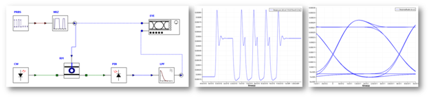
Figure 10: The test bench to measure the transient response of the device for a given operating point, modulation format and bitrate (left). The transient response showing the overshooting effect in the device dynamic response (center) and the eye diagram highlights the filtered overshoot as a source of penalty at the receiver stage (right).
For WDM interconnection systems ring modulators modulate only light at particular wavelengths and allow light at all other wavelengths to pass through the modulators without been affected [10]. Having determined the optimum operation point of the device, one can cascade several ring modulators with different resonant wavelengths on a single waveguide, and modulate different wavelengths of light independently. This multichannel large scale integrated circuit can be simulated with INTERCONNECT where the combined impact of the “overshoot” effect of each ring modulator can be easily evaluated.
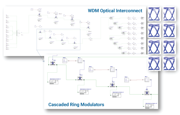
Figure 11: The circuit schematic and simulation results of an 8-channel WDM system interconnect with a comb laser as input. Cascaded ring modulators, in detail, allow for modulation and multiplexing of multiple WDM channels.
Summary
Verification of PICs is particularly challenging because it requires simulation of bidirectional opto-electronic elements that process digital, electrical and optical signals. Optical signals typically have to support multiple modes and multiple channels. Lumerical’s INTERCONNECT simulation framework can not only handle the complexity of different signal types but also offers frequency and time domain simulations, which are both complementary and indispensable when designing large scale photonic integrated circuits.
References
[1] A. Mekis, et al. “Computer-Aided Design for CMOS Photonics”. Silicon Photonics for Telecommunications and Biomedicine, First Edition, Edited by S. Fathpour and B. Jalali, CRC Press (2011).
[2] R. Nagarajan, et all. “Large-scale photonic integrated circuits,” Selected Topics in Quantum Electronics, IEEE Journal of , vol.11, no.1, pp.50,65, Jan.-Feb. 2005
[3] L. Thylén, et all. “The Moore’s law for photonic integrated circuits”, Journal of Zhejiang University SCIENCE A, Volume 7, Issue 12, pp 1961-1967. December 2006.
[4] J. Klein and J. Pond, “Simulation and Optimization of Photonic Integrated Circuits,” in Advanced Photonics Congress, (Optical Society of America, 2012)
[5] Lumerical Solutions. (2012). Lumerical Announces INTERCONNECT: A Robust, Configurable, Flexible Photonic Integrated Circuit Design Tool [Press release]. Retrieved from http://www.lumerical.com/company/news/releases/interconnect_photonic_integrated_circuit_design.html
[6] Z. Zhu and T. G. Brown, “Full-vectorial finite-difference analysis of microstructured optical fibers,” Opt. Express 10, 853–864 (2002)
[7] A. Taflove and S. C. Hagness, Computational Electrodynamics: The Finite-Difference Time-Domain Method, Third Edition. Artech House (2005).
[8] D. M. Pozar, Microwave Engineering, Third edition. John Wiley & Sons (2004).
[9] A. Ayazi, et all, “Linearity of silicon ring modulators for analog optical links,” Optics Express, Vol. 20, Issue 12, pp. 13115-13122 (2012).
[10] Q. Xu, et all, “Cascaded silicon micro-ring modulators for WDM optical interconnection,” Optics Express, Optics Express, Vol. 14, Issue 20, pp. 9431-9435 (2006).