

Introduction
Because of their compact footprint and potential for low drive-voltages, microring resonator modulators have attracted significant scientific and technological interest in recent years. This is especially true for silicon photonics [1], where passive silicon waveguide structures have shown an unprecedented reduction in footprint, including wavelength selective devices such as microring resonators. The INTERCONNECT [2] element library contains different elements that allows for building ring modulators as a composition of different primitives, such as phase shifters, waveguides and couplers. This composition of primitive elements or compound element offers tremendous flexibility to easily define new compact models using arbitrarily complex modulator sub-circuits. The INTERCONNECT element library also includes a ring modulator primitive element, facilitating the process of designing large scale photonic integrated circuits, where a compound element can be replaced by a single primitive element.
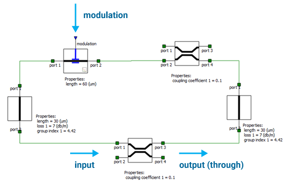
Figure 1: INTERCONNECT ring modulator compound element: the circuit is composed of phase shifting, waveguide and coupling elements
A static model can be used to simulate ring modulators, where the transmission function that represents the relationship between the input and through port is a function of the modulation voltage at a particular frequency of operation [3]. This model accounts for the modulation of the device, but it does not include the frequency dependent transfer function. The INTERCONNECT ring modulator model contains a time-varying frequency transfer function that represents the relationship between the input and through port. This quasi-static behavior allows for using the ring modulator not only as a modulator but also as a filter or multiplexer device when cascading multiple ring modulators. This approach is far more sophisticated than using static analysis, where the device behavior is only calculated at its frequency of operation. However, to properly simulate circuits that include ring resonators, a full dynamic analysis of the modulator may be required. To overcome the limitations of the quasi-static analysis the INTERCONNECT ring modulator element was extended to include full dynamic behavior.
Frequency-dependent microring transmission
We will start by describing the frequency-dependent transmission of the ring modulator, the basis for the time-domain quasi static model of INTERCONNECT. The resonator modulator configuration is depicted in Figure 2. A continuous wave (CW) incoming optical wave is modulated by varying the refractive index of the microring resonator. Different from Fabry-Perot resonators, ring resonators use couplers instead of mirrors for optical feedback.
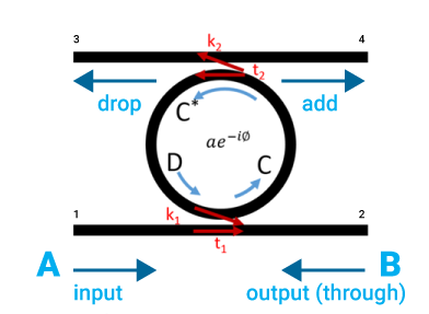
Figure 2: Schematic representation of a ring resonator modulator device.
From Figure 2, the field relationships are [3]:
| $$B = {t_1A+ik_1D} $$ | (1) |
| $$D = {t_2Cae^{-i \phi}} $$ | (2) |
| $$C = {ik_1A+t_1D} $$ | (3) |
Where A is the input optical field at port 1, and B is the output optical field (through) at port 2. a is the attenuation after each round-trip, t1 ,k1 and t2 ,k2 are the resonator transmission and coupling coefficients for the first and second coupler respectively. Phi (Φ) is the phase-shift after each round trip. Using a transfer matrix method, the static transmission is calculated as:
| $$T = {B \over A} = {t_1-t_2ae^{-i \phi} \over 1-t_1t_2ae^{-i \phi }} $$ | (4) |
In the frequency domain, the INTERCONNECT ring resonator primitive element calculates these parameters from the round trip length, the waveguide propagation properties and the coupling coefficients. Figure 3 shows the transmission of a 60 µm ring resonator. The exact same results are obtained if we build the ring resonator using primitive elements, showing the validity of the primitive ring model and equation (4).
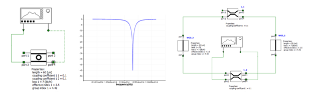
Figure 3: For the same set or parameters. The ring modulator primitive element (right) and compound element (left) have the same transmission function.
If we add time dependence to a and f we have a quasi-static model:
| $$T(t) = {B(t) \over A} = {t_1-t_2a(t)e^{-i \phi (t)} \over 1-t_1t_2a(t)e^{-i \phi (t)}}, \phi (t) = {2 \pi \over \lambda} \{ {n_{eff} + \Delta n_{eff} [v(t)] \}l} $$ | (5) |
Where l is the wavelength of operation, neff is the effective index, Dneff is the index change for a given voltage v at time instant t, and l is the round trip length. This means the transfer function of the ring modulator is time dependent. In the frequency domain, INTERCONNECT uses the steady-state value of the modulation voltage to define the device transfer function, allowing users to vary the DC or bias voltage and evaluate the device complex transfer function. Figure 4 shows the device transmission as a function of frequency and modulation voltage. From these results, different parameters such as extinction ratio and frequency detuning can be easily extracted.
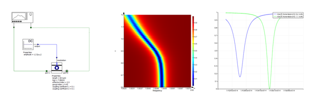
Figure 4: The frequency response of the ring modulator element as a function of input voltage allows for extraction of the extinction ratio and frequency detuning.
Time-dependent microring transmission
The INTERCONNECT ring modulator model implements equation (5) as a time-varying digital filter. The user can set the model to update or to interpolate filter coefficients. By selecting the update option the modulator will update the filter coefficient as function of time – this option is accurate but requires constant updating of filter coefficients. By selecting the interpolate option the modulator will pre-calculate the filter coefficients for a set of pre-defined input voltage values (v1, v2,…vN) at the beginning of the simulation, and it will interpolate coefficient values during the simulation – the accuracy of the interpolation depends on the number of pre-defined input voltage values and it does not require constant updating of the filter coefficients.
| $$T( \nu _1) = {t_1-t_2a(\nu_1)e^{-i \phi (\nu_1)} \over 1-t_1t_2a(\nu_1)e^{-i \phi (\nu_1)}}, T(\nu_2) = {t_1-t_2a(\nu_2)e^{-i \phi(\nu_2)} \over 1-t_1t_2a(\nu_2)e^{-i \phi (\nu_2)}},…, T(\nu_N) = {t_1-t_2a(\nu_N)e^{-i \phi(\nu_N)} \over 1-t_1t_2a(\nu_N)e^{-i \phi (\nu_N)}}$$ | (6) |
Figure 5 depicts a ring modulator circuit, where the modulator is driven by a 25 GBs NRZ signal (0.6 to 1 Volt). The modulated output signal shows that the quasi-static model does not include the cavity dynamics of the device, which in some cases can be ignored depending on the input modulation speed and the quality factor of the modulator.
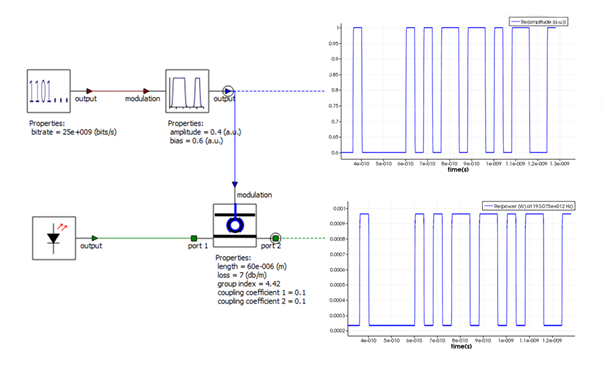
Figure 5: Ring modulator circuit (primitive element): the modulator is driven by a 25 GBs NRZ signal (0.6 to 1 Volt). The modulated optical signal does not include the cavity dynamics of the modulator.
This quasi-static model models the steady-state property of the resonator and does not take cavity dynamics into account. Depending on the Q-factor and modulation speed the dynamics of the ring modulator will have to be taken into account [4]. One option to include the full dynamic behavior of the modulator is to build the ring resonator using primitive elements, and evaluate if the steady-state model is adequate to simulate the current circuit under test [5]. Figure 6 compares the output waveform of the primitive element (quasi-static) and the dynamic model with the same parameters as Figure 5. The figure shows that for this ring modulator (Q-factor ~ 5000) and with this modulation speed a fully dynamical analysis of the modulator is required.
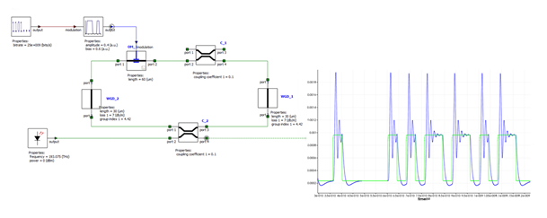
Figure 6: Comparison between the modulated output signal from the compound element (blue) and the primitive element (green)
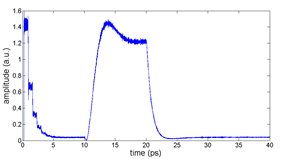
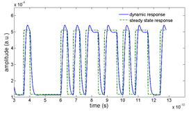
Figure 7: The steady-state and dynamic response of the ring modulator in a circuit level simulation (left) and the dynamic response of a ring modulator simulated using a 2.5D FDTD method with a time-varying refractive index (right).
The overshoot and ringdown behavior, seen in Figure 6, is expected when one considers the dynamics of the cavity resonance. When the cavity is on resonance, optical energy is stored in the high Q ring. As the cavity is brought out of resonance, the energy stored in the ring must be released. To verify the results of the INTERCONNECT compound model, a component level simulation using a 2.5D FDTD method [6] was carried out to verify this response. This method is ideal for optically large planar components because it offers comparable accuracy to 3D FDTD while only requiring the simulation time and memory of a 2D FDTD simulation. By introducing a refractive index that varies in time, we can observe the dynamic response of the ring modulator to an input electrical signal. For the same ring design, Figure 7 shows the results of the INTERCONNECT model to a bit sequence and the result of the 2.5D FDTD model when a step index ∆n is applied between 10ps and 20ps. We see that the overshoot and ringing effect calculated by the INTERCONNECT model is very similar to what is calculated by the full 2.5D FDTD simulation.
In order to facilitate the process of designing large scale photonic integrated circuits, the INTERCONNECT ring modulator primitive element model was extended to support full dynamic behavior by solving the following time domain field equations [3]:
| $$B(t) = {t_1A+ik_1D(t)} $$ | (7) |
| $$D(t) = {C(t- \tau)a(t)e^{-i \phi (t)}} $$ | (8) |
| $$C(t) = {t_2 (ik_1A(t)+t_1D(t))} $$ | (9) |
Where t is the resonator round-trip delay time. By using a traveling wave model to simulate (7-9), the new primitive model can now model the static, quasi-static and dynamic behavior of micro-ring modulators. Figure 8 shows the output modulated signal of the new dynamic model, where the results obtained are the same as if using an equivalent compound element.
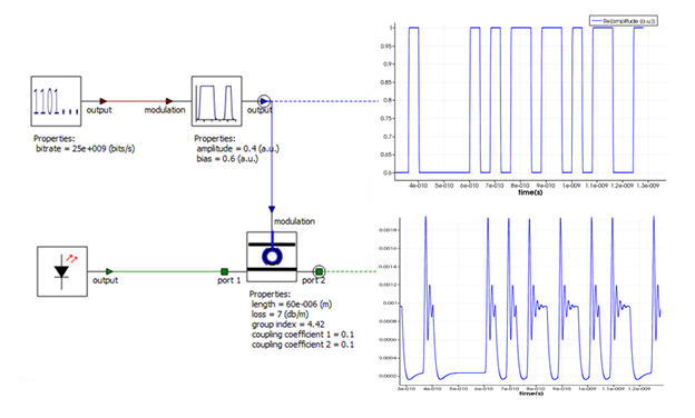
Figure 8: Ring modulator circuit (primitive element): The modulated optical signal now include the cavity dynamics of the modulator.
Summary
The INTERCONNECT ring modulator element allows for static, quasi-static and full time dependent analysis of microring resonators, allowing for fast and accurate simulation of large scale photonic integrated circuits.
References
[1] W. Bogaerts, et all. “Silicon microring resonators”, Laser & Photon. Rev., Vol. 6, No. 1. , pp. 47-73. January 2012.
[2] Lumerical Solutions. (2012). Lumerical Announces INTERCONNECT: A Robust, Configurable, Flexible Photonic Integrated Circuit Design Tool [Press release].
[3] W. Sacher and J. Poon, “Dynamics of microring resonator modulators,” Opt. Express 16, 15741-15753 (2008).
[4] A. Ayazi, et all, “Linearity of silicon ring modulators for analog optical links,” Opt. Express 20, 13115-13122 (2012).
[5] James F. Pond, et all. ” A complete design flow for silicon photonics “, SPIE Photonics Europe, p.9133-39 (2014).
[6] Lumerical Solutions. (2014). Lumerical’s 2.5D FDTD Propagation Method [Knowledge Base]. Retrieved from https://www.lumerical.com/solutions/innovation/2.5d_fdtd_propagation_method.html