

Abstract
Certain FDTD material models such as nonlinear, negative index, or multi-level multi-electron gain models are challenging to provide in commercial software because of the flexibility that is required. A nonlinear model may be as simple as an instantaneous χ(2) or χ(3) effect, or may involve additional dispersive and anisotropic nonlinear terms. While it is relatively straightforward to provide a particular nonlinear material model appropriate for a specific application, it is a challenge to provide the wide range of different nonlinear material models that are required in general. In addition, it can be challenging to combine nonlinear responses with linear dispersion, which can be critical when considering issues such as phase matching. Lumerical’s Flexible Material Plugins provide a solution to these challenges and allow for end users or Lumerical, working either independently or in collaboration, to develop new electric and magnetic FDTD material models.
The plugins are implemented in FDTD Solutions and the 2.5D FDTD Propagator in MODE Solutions. The same plugins can be used for both products. While FDTD Solutions provides the most accurate method for 3D nonlinear simulation, the simulation times are often much longer than for linear systems and this can be prohibitive for larger geometries. For nonlinear and gain effects in waveguides, MODE Solutions can quickly simulate large nonlinear waveguide components.
In this whitepaper, we provide an implementation summary that explains how the material plugin works, followed by several application examples including nonlinear, gain, and negative index applications.
Implementation summary
We summarize the key aspects of the material plugin implementation. Additional implementation details along with several examples can be found in the FDTD Solutions Knowledge Base section on user-defined materials.
The field update
The formulation by Lumerical requires C++ code that solves the following equation for En:
$$U^nE^n + {P^n \over \epsilon_0} = V^n $$
where En is the electric field at time nΔt, Pn is the desired polarization at time nΔt and Un and Vn are input values that we provide. For example, in the trivial case of a non-dispersive linear medium, we haveP n=χEn and the user would write a one line function that returns:
$$E^n = {V^n \over {U^n + \zeta}}$$
A similar equation needs to be solved to introduce any desired magnetization.
The use of the variables U and V allow us to add the polarization P to any desired base material, which makes it possible to easily combine nonlinear and gain effects with Lumerical’s Multi-Coefficient Materials (MCMs) for the linear dispersion.
Material parameters
The end user can specify any number of parameters for the material. For example, the user might want to specify parameters χ(2) or χ(3). These parameters appear in the GUI user interface and can be easily modified by the end user.
Anisotropic materials
The user can provide different parameters for each component of the electric and magnetic field, or even different updates for each component. Therefore materials with diagonal anisotropy can be easily introduced.
Auxiliary fields
Many updates require a number of auxiliary fields that must be stored and updated from one time step to the next. For example, a multi-level, multi-electron model must store and update level populations. The user can indicate how many storage fields are required and can then update them, and can also monitor these fields in the GUI.
Interfaces between media
When a plugin material is on the interface of two media, the user has two options which can be set on a material by material basis:
The solver can revert to using the base material for Yee cells that contain an interface. This is appropriate when the polarization, P, introduced by the plugin can be seen as a small perturbation on the polarization of the base material.
The solver can revert to staircase meshing whenever the plugin material is encountered at an interface. This is appropriate when the polarization implemented by the plugin is not a small perturbation of the base material.
Limitations
We summarize some of the limitations of the current plugin implementation below. Lumerical is always interested in learning about use cases where these limitations make it impossible to achieve specific simulation goals.
Non-diagonal anisotropy
The current implementation of the Flexible Material Plugin does not provide the information on all field components that is necessary to directly handle off diagonal anisotropy. This is in fact a challenging aspect of FDTD simulations because, in the Yee cell the different field components are positioned at different spatial locations. An alternative solution however is provided by another feature of Lumerical’s software, which can be applied to the E field update only. The user can provide any spatial rotation, or even a more general unitary transformation, to rotate the E field into a different reference frame, and this transformation can also be spatially varying. While there is no general method to diagonalize the nonlinear susceptibilities, there are some situations where this transformation can be used.
Non-local effects
The current implementation does not allow for non-local effects. This would require knowledge of the neighboring field components, which is not currently available.
Compatibility with Conformal Mesh Technology
Conformal Mesh Technology can resolve interfaces with sub-mesh cell accuracy by specially treating the E and H fields at interfaces to solve an integral form of Maxwell’s equations. It is not possible to introduce plugin materials in the current version that can also be used with a conformal mesh update. However, as mentioned previously, the user can choose to revert to the base material for Yee cells containing an interface, and the base material can be used with the conformal mesh update.
Application Examples
Second harmonic generation
We show second harmonic generation in a simple setup where a plane wave is incident on a thin slab of nonlinear silicon. The source wavelength is 1500nm and we monitor the field as a function of time in transmission and, by Fourier transform, we can easily plot the transmitted spectrum. We compare two examples: (a) we use a constant dielectric material to represent the linear silicon response and (b) we use a dispersive multi-coefficient mode (MCM) for silicon. Both results show second harmonic generation at the expected wavelengths, however, the short wavelength harmonics have a significantly lower amplitude in the dispersive silicon case because the silicon is increasingly absorbing below about 1000nm. More details can be found in the section on harmonic generation in the FDTD Solutions Knowledge Base.
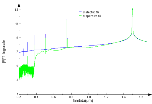
Figure 1: We compare the second harmonic generation for nonlinear silicon where (a) the linear silicon properties are represented as a simple dielectric (“dielectric Si”) and (b) where the linear silicon is more accurately represented using Lumericals MCM (“dispersive Si”). There is suppression of the harmonics at shorter wavelengths due to the high absorption of silicon, an effect that is not captured with a simple dielectric model.
χ(3) Raman and Kerr
We have created a χ(3) material that includes both Raman and Kerr effects. This material can be used to model soliton formation in an SOI waveguide. To solve this problem, we first calculate the effective index of the waveguide over a broad wavelength range. We can then run a 1D FDTD simulation using an effective dispersive material, which can be accurately fitted with the MCM, and add the desired nonlinear effects. In the figure below, we can observe the formation of solitons as the light propagates over several millimeters. Details and simulation examples can be found in the FDTD Solutions Knowledge Base section on solitons in SOI waveguides.
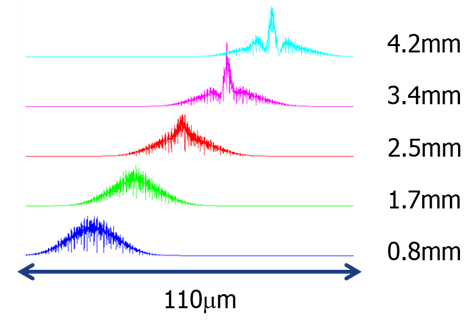
Figure 2: We can see the electric field intensity (plotted over 110μm) as the light propagates several mms down a nonlinear SOI waveguide, showing the process of soliton formation. Initially, the light retains the Gaussian shape of the source, however, by 4.2mm the pulse has reshaped and contracted.
Four wave mixing
An SOI based ring resonator, as shown below, can be used to see four wave mixing (FWM) when a Raman and Kerr χ(3) nonlinearity is introduced. The effect can be greatly enhanced at resonant wavelengths because the field intensity in the ring becomes higher, and the effective propagation length can be long. In addition, the ring resonator has resonances that are separated by a constant frequency difference, which makes it an ideal component for FWM.
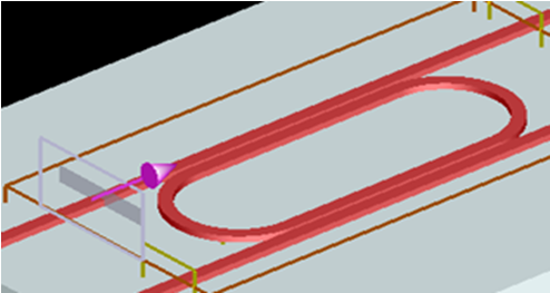
Figure 3: A racetrack ring resonator that can be used for FWM.
In this simulation, the structure is tuned to have resonances at the pump and signal wavelengths, therefore the converted light will also be on resonance. The figure below shows the output spectrum where we can clearly see the converted signal. While the conversion efficiency is still low, this clearly demonstrates that FWM can be simulated. More details and example files are available in the FDTD Solutions Knowledge Base section on four-wave mixing.
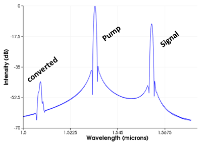
Figure 4: The intensity vs wavelength on a dB scale, showing the pump and signal wavelengths which are sources in the simulation. In addition, we see the converted signal which has been created from the pump and signal by FWM.
Bulk negative index
The material plugin makes it possible to update both the electric polarization and magnetic magnetization. With this capability, we have created an electric and magnetic Lorentz medium. With a suitable choice of parameters for the Lorentz models, we can achieve a negative permittivity and permeability at the same wavelength. This makes it possible to simulate the unusual refraction that occurs for a bulk negative index medium, shown in the figure below for a slab of this medium.
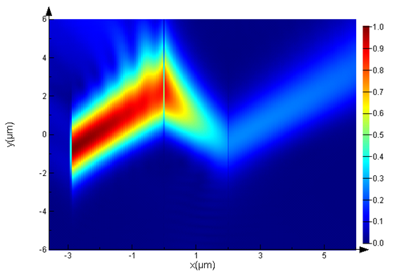
Figure 5: Negative refraction that occurs in a slab of a negative index medium.
Gain media and lasing
The material plugin makes it possible to introduce sophisticated material models such as a four-level, two-electron model. The level diagram below shows a model that we have implemented that is distributed with the software. Using this model we can perform pump-probe simulations, simulate lasing in 1D cavities, or even consider more complex devices such as the optically-pumped microdisk laser example below. It is also possible to create a plugin material that is electrically pumped and lasing is achieved through spontaneous emission.
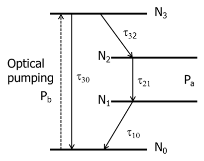
Figure 6: The level diagram for a four-level two-electron system. In this figure, we consider optical pumping, but it is possible to extend the model to include electrical pumping and spontaneous emission.
We can quickly simulate a laser made from a microdisk gain medium coupled with a waveguide using 2D FDTD. The medium is optically pumped through the waveguide at 1200nm, and lases at 1500nm. We can look at dynamics of the onset of lasing as the resonant mode is established, and we can also monitor the level populations at different locations. These results are shown in the figures below. More details and example files can be found in the microdisk laser example in the FDTD Solutions Knowledge Base.
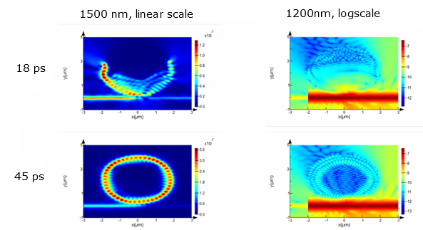
Figure 7: The electric field intensity at different times as the lasing mode is established. The lasing occurs at 1500nm and is shown on a linear scale, while the pump is at 1200nm and is shown on a log scale.
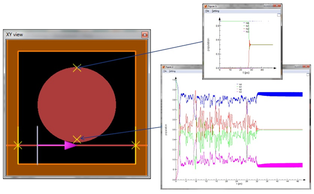
Figure 8: The level populations shown at different points on the disk. The point close to the waveguide is immediately affected by the pump signal and has chaotic behavior until the lasing mode is established and a small, stable population inversion is achieved. The point on the far side of the disk is unaffected until just before the lasting mode is established and also achieves a small population inversion.
Optical bistability
Nonlinear Kerr effects can lead to bistability in ring resonators, meaning that the normalized output intensity of the ring changes as the source intensity is modified and the output depends on whether we are increasing or decreasing the source intensity. Simulated results of optical bistability are shown in the figure below for the structure defined in X. Wang, H. Jiang, J. Chen, P. Wang, Y. Lu and H. Ming, “Optical bistability effect in plasmonic racetrack resonator with high extinction ratio”, Optics Express, Vol. 19, No. 20, 2011.
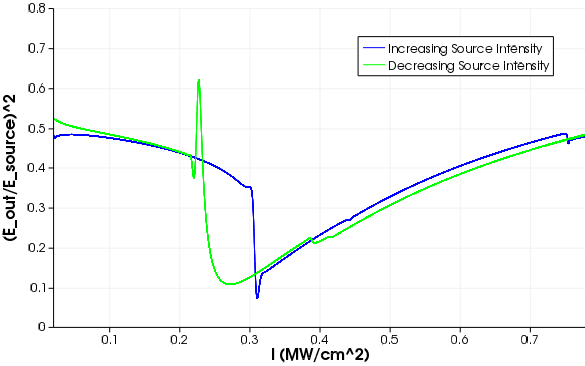
Figure 9: The curve of normalized output intensity vs source intensity for a bistable ring resonator. We can see that the normalized output intensity not only depends on the source intensity, as expected for a Kerr nonlinearity, but also exhibits bistable behavior where the two curves are different depending on whether the source intensity is increased or decreased.
Time dependent refractive index
Electro-optical ring modulators can be made by using carrier injection to electrically modify the refractive index (and loss) of a waveguide which results in a small phase change as light propagates in the waveguide. By inducing this small, electrically controlled phase change it is possible to modulate an optical signal in a ring modulator by bringing the ring in and out of resonance electrically. If a high Q ring is on resonance there is a relatively large amount of optical energy stored in the ring. When the ring is brought out of resonance, the energy stored in the ring must be released. This leads to an interesting overshoot effect which can limit the maximum modulation speed.
Using the material plugin, we can create a section of a ring with an index that changes as a step function in time and simulate the effect of injecting carriers electrically. With MODE Solutions, we can quickly simulate a ring modulator for long enough to consider a single step function. In the figure below, we can clearly see the overshoot effects that occur on the rising edge when the ring is suddenly brought out of resonance. On the falling edge, the ring is being brought into resonance and therefore we see much less of an effect.
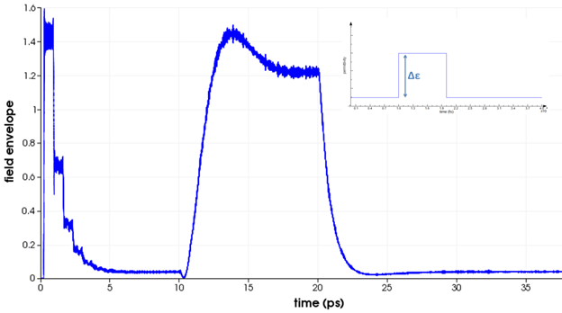
Figure 10: The output field intensity of a ring modulator that is subject to the step change in index that is shown in the upper right inset which brings the ring out of resonance, then back into resonance. We clearly see the overshoot effect that occurs when the ring is brought out of resonance because the optical energy stored in the ring must be released.
Conclusions
Lumerical’s Flexible Material Plugin makes it possible for end users, either alone or in collaboration with Lumerical, to develop sophisticated electromagnetic material models that run within our industry leading FDTD solvers. This makes it possible to simulate a wide range of effects including nonlinearities, gain media, negative index media, and time dependent refractive index changes. We look forward to collaborating with our end users to continue to develop and share new material models for leading-edge applications.