

Lumerical’s 2.5D variational FDTD (varFDTD) solver offers more accuracy and versatility than beam propagation method (BPM) for the virtual prototyping of planar integrated optical components
Lumerical MODE Solutions’ variational FDTD (varFDTD) solver efficiently simulates the propagation of optical radiation in a wide array of guided structures, from ridge waveguide-based systems to more complex geometries such as photonic crystals. Its ability to predict the performance of optically large components more accurately than beam propagation methods, combined with its optimized computation engine, renders it a robust waveguide design environment well suited for the virtual prototyping and optimization of planar integrated optical components and circuits.
Background
The finite-difference time-domain (FDTD) technique is one of the most versatile and accurate methods for simulating light propagation in nanoscale components. However, when applied to three-dimensional structures, FDTD is highly computationally intensive, making it difficult to treat large integrated optical components efficiently. There are several alternative methods for simulating wave propagation over large distances: the well-known Beam Propagation Method (BPM) relies on a slowly varying envelope assumption and can simulate large structures quickly. However, its accuracy is compromised for propagation at large angles, or in components with high refractive-index contrast. The more rigorous Eigenmode Expansion Method (EME) is ideal for treating bi-directional propagation, but can be inefficient for simulating omni-directional propagation due to the large number of modes required to achieve sufficient accuracy.
In contrast to traditional propagation methods, the varFDTD method in MODE Solutions allows for the broadband modeling of linear and non-linear phenomena in planar waveguide systems, without making any assumptions about an optical axis, device geometry, or the materials used. For planar waveguide components, the varFDTD method offers comparable accuracy and versatility to that of 3D FDTD, while only requiring the simulation time and memory of a 2D FDTD simulation. Combined with MODE Solutions eigenmode solver and bidirectional igenmode expansion (EME) solver, MODE Solutions is the ideal tool for virtual prototyping of large integrated optical components, reducing the need for expensive, time-consuming manufactured prototypes.
varFDTD offers the best trade-off between speed and accuracy for omni-directional in-plane propagation
The varFDTD solver is ideal for simulating omni-directional light propagation in optically large planar integrated optical components. The method involves reducing the 3D problem into an effective 2D problem by converting the vertical waveguide structure into effective dispersive materials that simultaneously account for material and waveguide dispersion, as illustrated in Figure 1.
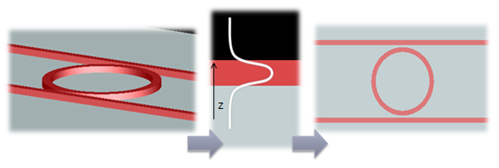
Figure 1. The vertical slab mode is used to collapse the 3D planar geometry into a 2D set of effective dispersive materials
There are currently two approaches for collapsing the geometry with the varFDTD solver:
- a variational procedure based on Hammer and Ivanova [1]; and
- a procedure based on the Reciprocity Theorem, as described in Snyder and Love [2].
In both cases, the key assumption is that there is negligible coupling between the different slab modes supported by the vertical waveguide structure. For many devices, such as SOI-based slab waveguide structures that only support two vertical modes with different polarizations, this is a very good assumption. In this case, the varFDTDcan provide results comparable to 3D FDTD using only the simulation time and memory of a 2D FDTD simulation. This provides designers with the opportunity to iterate through many design parameters efficiently, as well as the ability to simulate components that are too large to be treated with 3D FDTD.
Ring resonator example: 2D speed with 3D accuracy
We will use a simple ring resonator to demonstrate the operation of MODE Solutions’ varFDTD solver.
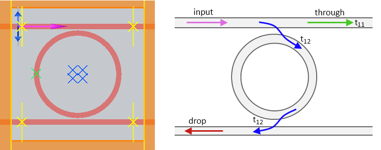
Figure 2. A four-port ring resonator.
MODE Solutions will automatically collapse the 3D geometry into a 2D set of effective materials. Note that the generated effective materials are also dispersive, where the dispersion comes both from the original material properties as well as the slab waveguide geometry. These generated materials are then fitted using Lumerical’s proprietary Multi-Coefficient Materials model into a form amenable for simulation via the FDTD algorithm.
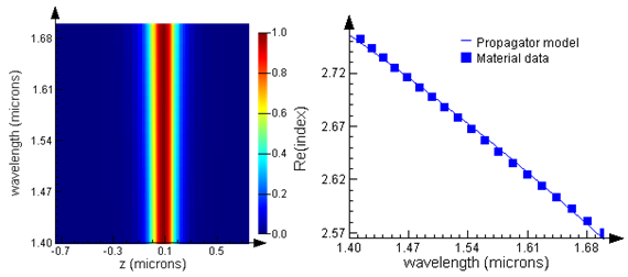
Figure 3. (left) Waveguide dispersion can be seen in the vertical slab mode profile (shown as a function of the vertical dimension z and wavelength). (right) The generated effective materials contain both waveguide dispersion from the slab waveguide geometry as well as material dispersion from silicon.
Once the 2D effective materials are generated, one can proceed with a 2D FDTD simulation using Lumerical’s optimized computation engine, which allows for parallel computation on multi-core processors and multi-node high performance computing systems.
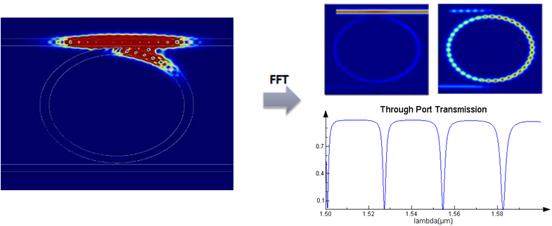
Figure 4. 2D FDTD simulation using the 2D effective materials gives broadband response with one simulation in the time domain.
Using built-in eigenmode expansion monitors, high resolution and high accuracy broadband transmission data into an arbitrary waveguide mode can be obtained in a single simulation. The signal transmitted into the fundamental mode at the through port is shown in FIGURE 5, which shows that the varFDTD method agrees very well with the 3D FDTD result, and is 100 times faster as shown in TABLE 1. FIGURE 5 also compares 2D FDTD (where the refractive index used is simply the effective index of the vertical slab mode) and 3D FDTD, and we can see that the agreement is poor. In particular, the key quantities we typically extract from such a simulation, the bandwidth and free spectral range (FSR), are very accurately calculated with the varFDTD method, which is not the case with the standard 2D FDTD approach. To facilitate comparisons between varFDTDD, 2D and 3D FDTD, in both plots of FIGURE 5, the varFDTD and 2D FDTD transmission spectra have been shifted so that the center peaks are aligned with the 3D FDTD result. In reality, precise positioning of this peak is achieved through thermal tuning.
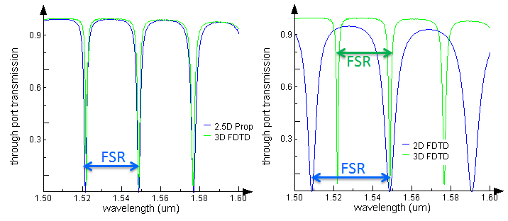
Figure 5. (left) Transmission into the fundamental mode at the through port obtained from a varFDTD simulation and a 3D FDTD simulation. (right) The same plot showing the result from a standard 2D FDTD approximation and 3D FDTD.
| Simulation Type | Memory | Processing time on a 2010 Intel Core i7 machine |
| 2D FDTD | 15MB | ~12 seconds |
| 2.5D FDTD | 18MB | ~15 seconds |
| 3D FDTD | 338MB | ~1500 seconds |
Table 1: Summary of the simulation time and memory required for the ring resonator example. In this case, 2D FDTD and varFDTD run at about 100 times faster than 3D FDTD.
Based on the accuracy and speed of computation available with the varFDTD solver, one can go a long way towards optimizing the ring resonator with MODE Solutions. And since simulations with ring resonators and other silicon photonic devices will typically require much larger simulation regions and longer simulation times, this varFDTD Solver can become invaluable for optimizing designs of this level of complexity.
Based on the accuracy and speed of computation available with the varFDTD solver, one can go a long way towards optimizing the ring resonator with MODE Solutions. And since simulations with ring resonators and other silicon photonic devices will typically require much larger simulation regions and longer simulation times, this varFDTD Solver can become invaluable for optimizing designs of this level of complexity.
varFDTD has the versatility to address a wide range of applications
Planar Tapers
With the varFDTD solver, it is trivial to accurately determine the broadband transmission into multiple modes of a wide taper. Because collapsing the vertical structure into an effective slab works perfectly well in a wide region like that of the taper, no approximations are made for light propagation in the waveguide slab and one can get results very close to 3D FDTD with this variatonal FDTD treatment.
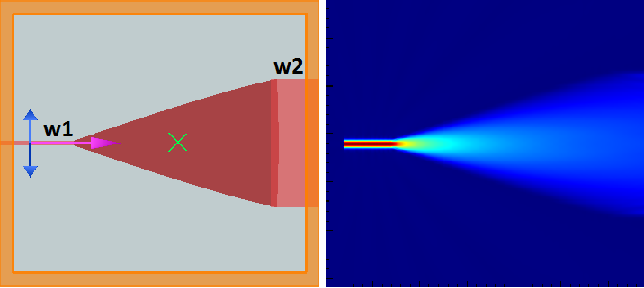
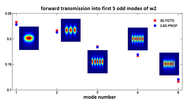
Figure 6. varFDTD simulation of a SOI waveguide taper. The shape of the taper was parameterized by w(x)= 〖α(L-x)〗^m+w_2 and optimized using the built-in optimization framework within MODE Solutions. The lower plot shows the transmission at a wavelength of 1550 nm into the first 5 even TE modes of waveguide 2.
Arrayed Waveguide Gratings (AWGs)
AWGs are essential for dense wavelength division multiplexing in optical networks. The size and complexity of these devices, as well as their sensitivity to phase errors, can make AWGs challenging for many propagation methods. With MODE Solutions’ varFDTD solver, one can obtain accurate broadband results with a single simulation.
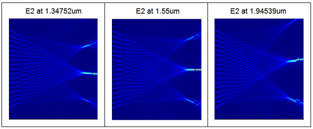
Figure 7. Wavelength dependent de-multiplexing can be seen in the output star coupler of the AWG simulated using the varFDTD solver. These results were all obtained from a single simulation in the time domain.
Nonlinear Waveguides
Simulating nonlinear effects in waveguides often require long simulation times and propagation lengths. The varFDTD solver combined with the flexible material plugins available within MODE Solutions is capable of simulating wave propagation over long distances efficiently, while still being able to accurately capture the interplay between the linear and nonlinear effects. The flexible material plugins are constructed via an open framework that allows end-users to develop their own models, tailored to their unique needs, in native C/C++/FORTRAN as dynamically linked library plugins. Those plugins can be used in combination with the multi-coefficient material models to simulate complicated nonlinear materials as shown in Figure 8.
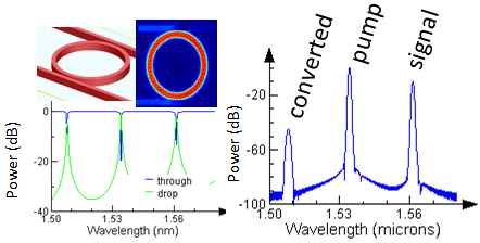
Figure 8. 2.5D FDTD simulation of four-wave mixing (FWM) in a nonlinear ring resonator. (left) The linear through and drop power. (right) Spectrum showing the pump, signal and converted light.
Conclusions
MODE Solutions’ varFDTD solver is a versatile solver for simulating broadband, omni-directional light propagation in waveguide components. For planar geometries where there is negligible coupling between different slab modes, varFDTD can provide results comparable to 3D FDTD using only the simulation time and memory of a 2D FDTD simulation. Combined with MODE Solutions eigenmode solver and bidirectional eigenmode expansion (EME) solver, MODE Solutions is the ideal tool for virtual prototyping of large integrated optical components, reducing the need for expensive, time-consuming manufactured prototypes.
References
[1] Manfred Hammer and Olena V. Ivanova, MESA Institute for Nanotechnology, University of Twente, Enschede, The Netherlands “Effective index approximation of photonic crystal slabs: a 2-to-1-D assessment”, Optical and Quantum Electronics ,Volume 41, Number 4, 267-283, DOI: 10.1007/s11082-009-9349-3
[2] Allan W. Snyder and John D. Love, Optical Waveguide Theory. Chapman & Hall, London, England, 1983.